Best in Class Widgets#
The following is a selection of several complex widgets that you can use to create dashboards for Supervisors, Managers, and Analysts.
Productive vs Indirect Time Widget#
Indirect time is a major source of avoidable labor cost. A Productive vs Indirect Time widget can help managers see what portion of the day is spent on non–value-add tasks. This widget dives deeper into the Utilization metric to help visualize where indirect hours are taking up the most space This can be done at the warehouse, shift, activity or user level.
Widget Type#
Pie chart, Stacked Bar
Steps#
Navigate to Widget Builder and click New.
Fill in basic widget details and select a data source that includes Measured time and Unmeasured time for warehouse, activity, or user. For this example, we’ll create the widget at the warehouse level.
Filter the data at the Filter stage. Include a date field.
Assign fields at the Fields stage.
Create a Pie chart in Chart Designer. Choose from the following options:
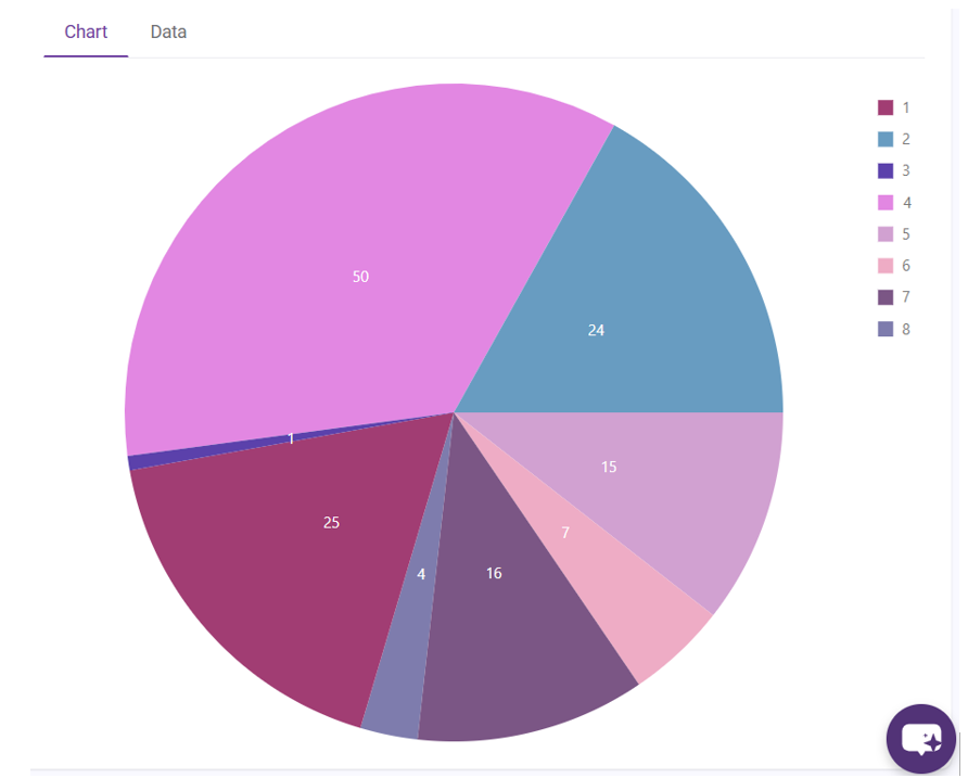
Set your Warehouse Code as the argument and Unmeasured time as the series to see which warehouses have the highest percentpercentage of indirect hours. If one warehouse has a disproportionate number of Indirect hours, you can then figure out why. In this example, Warehouse 4 has more indirect hours than any other warehouse, and warehouse 3 has the least.
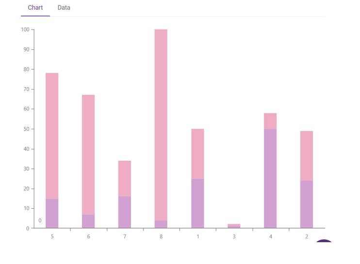
Create a stacked bar chart that shows a percentage of unmeasured time vs measured time per warehouse. We can see that Warehouse 4 had more Indirect hours than any other warehouse and has the highest disparity between productive and indirect activities. However, this chart also tells us that while Warehouse 3 does have the least number of indirect hours, Warehouse 8 has the best ratio.
How to Interpret Productive vs Indirect Time Widget Results#
This widget helps you visualize how labor is being spent between Productive time (direct work contributing to output) and Indirect time (required but non–value-add or not captured in standards).
Watch for:
One warehouse with a much larger indirect portion than others. This indicates a local issue worth investigating.
Large swings day-to-day. This indicates inconsistency in staffing, downtime, or workload distribution.
Indirect time appears low, but performance/utilization is poor. This indicates misclassification of time or missing labor tracking.
Labor Performance by Warehouse#
Chart Type
Drill-Down Bar Chart
Overview#
This widget pulls real-time data across multiple sites and allows drilling down into individual performance. You can easily compare warehouse performance, then drill into shifts and individuals to quickly identify strengths and bottlenecks.
Data Requirements#
Warehouse-level performance data
Activity and/or Shift level data
Individual user-level performance data
Setup Procedure#
Let’s set up a drill-down widget that starts at the Warehouse performance at the top level, then by Shift, then by Activity, then by User. You can click on individual warehouse data to show the shift data for that warehouse, then click on each shift to show the individual activity data, and finally click on an activity to show data for each user.
This requires 4 separate widgets for each dataset we want represented. The first three should be bar charts, with the final one (user data) being a grid. Each widget in this example requires their own set of parameters, plus the parameters from the widget level above it. Look at the table below to see an example of what parameters are needed.
Widget |
Widget Type |
Parameters |
|---|---|---|
Warehouse |
Bar |
MIN_STOP_DATE_LOCAL, WAREHOUSE_CODE |
Shift |
Bar |
MIN_STOP_DATE_LOCAL, WAREHOUSE_CODE, SHIFT |
Activity |
Bar |
MIN_STOP_DATE_LOCAL, WAREHOUSE_CODE, SHIFT, ACTIVITY |
User |
Grid |
MIN_STOP_DATE_LOCAL, WAREHOUSE_CODE, SHIFT, ACTIVITY, USER_NAME |
Navigate to Widget Builder. Build 4 widgets with the respective parameters listed above. For details on how to create widgets, refer to the Creating Widgets section of the Help Center.
Create a Drill-Down path with the Warehouse data at the top level. Refer to Drill Down Paths.
Add the widget to a dashboard to track performance.
Metrics Summary by Employee#
Chart Type#
Cascading Grid Chart
Overview#
This is a cascading widget that provides leaders with an employee-level performance summary. This enables leaders to coach employees effectively with clear performance comparisons.
Data Requirements#
Warehouse-level performance data
Employee performance data
Team or group data
Benchmarks for expected performance
Setup Procedure#
Let’s set up a cascading widget that has warehouse- level metrics in the root widget, and employee data in its child widgets. Leaders open the dashboard and see:
Warehouse-level KPIs (root widget)
Employee performance summaries (child widgets)
When you click a warehouse, all child widgets instantly filter to employees in that warehouse.
Widget |
Widget Type |
Parameters |
|---|---|---|
Warehouse Performance Overview |
Grid |
MIN_STOP_DATE_LOCAL, WAREHOUSE_CODE |
Shift Summary |
Bar |
MIN_STOP_DATE_LOCAL, WAREHOUSE_CODE, USER_NAME, USER_GROUP, BASE_SHIFT |
Individual User Performance |
Bar |
MIN_STOP_DATE_LOCAL, WAREHOUSE_CODE, USER_NAME, USER_GROUP, BASE_SHIFT |
Navigate to Widget Builder. Build the Warehouse-level root widget and the Employee-level child widgets using the parameters outlined in your design. Ensure each child widget includes all parameters of the root widget. For details on how to create widgets, refer to the Creating Widgets section of the Help Center.
Create a Cascading Widget Group with Warehouse data as the root widget. Go to Admin Tools> Widgets >Cascading Widget Configuration, and create a new group. Assign the Warehouse Performance widget as the root and add the Employee-level widgets as child widgets. Refer to the Cascading Widget Groups procedure in the Help Center.
Add the cascading widget group to a dashboard to track performance.
Indirect Hours by Warehouse#
Chart Type#
Drill-Down pie chart
Overview#
This pie chart is a view into how many hours are being attributed to different indirect tasks. It informs the team where there is waste and barriers in the operation and keeps these issues from lowering performance KPIs. Reminder that an indirect hours are time spent by employees on non-essential, non-productive activities. E.g., meetings, breaks, lunch time.
Data Requirements#
Indirect activity data
Hours logged per warehouse per task
Performance benchmarks
Setup Procedure#
Let’s build a widget that allows you to see Indirect Hours by warehouse and find which warehouse, specific indirect activities, and even users are contributing the most hours. This configuration creates a drill-down widget that begins with a high-level view of Indirect Hours by Warehouse, then drills into a detailed user-level grid for deeper analysis. You can click on a warehouse segment in the pie chart to reveal the indirect activities, then click again to see individual users contributing indirect hours within that warehouse and review supporting data such as user group and shift.
Widget |
Widget Type |
Parameters |
|---|---|---|
Indirect Hours by Warehouse |
Pie |
MIN_STOP_DATE_LOCAL, WAREHOUSE_CODE |
Indirect Hours by Activity |
Pie |
MIN_STOP_DATE_LOCAL, WAREHOUSE_CODE, USER_NAME, USER_GROUP, BASE_SHIFT |
Individual User Performance |
Grid |
MIN_STOP_DATE_LOCAL, WAREHOUSE_CODE, USER_NAME, USER_GROUP, BASE_SHIFT |
Navigate to Widget Builder. Build 3 separate widgets with the respective parameters listed above. For details on how to create widgets, refer to the Creating Widgets section of the Help Center.
Create a Drill-Down path with the Warehouse data at the top level. Refer to Drill Down Paths in the Help Center.
Add the widget to a dashboard to track performance.
Overtime Hours by Employee#
Chart Type#
Stacked Bar Chart
Overview#
This widget tracks overtime hours per employee. When connected to time and attendance systems, this widget can generate alerts to help limit overtime costs.
Data Requirements#
Time clock or attendance data
Regular vs. overtime hours
User-level labor assignments
Setup Procedure#
Let’s set up a widget that will show total hours worked per employee. The hours will be grouped into regular and overtime hours. Regular hours are colored green. If an employee works overtime, the extra hours will appear yellow. If an employee works an excessive amount of overtime, the extra hours appear red.
Navigate to Widget Builder. Build your widget using employee timesheet data, overtime data, and standard shift data. For details on how to create widgets, refer to the Creating Widgets section of the Help Center.
Build a stacked bar chart. To add the different colored sections, add multiple series. Refer to to Setting Up Stacked Bar Charts the Help Center.
Add the widget to a dashboard to track performance.
Note
It’s possible to integrate this chart into a drill down from the warehouse or shift level. Refer to Drill Down Paths in the Help Center.
Forecast Demand by Labor Category and Shift#
Chart Type#
Line Chart
Overview#
This widget projects staffing needs by labor category and shift by combining forecasted demand with labor planning inputs. It follows the same process described in Creating Widgets Based on Labor Planning Results, including how to extract values from object arrays and build calculated fields.
Data Requirements#
Forecasted demand data
Labor categories (e.g., pickers, packers, forklift drivers)
Planned shift structures
Setup Procedure#
Let’s make a widget that predicts the number of hours needed on a daily basis to cover the forecasted workload demand each week. This widget will use previous data metrics to predict future labor demands using the Labor Planning module.
Create a new widget in non-guided mode and select LP FORECAST RESULTS as your data source. Apply filters such as date range, warehouse/site, and demand type as needed.
Add a Display Fields stage and convert required arrays using the same method described in Converting Object Arrays into Separate Data Columns.
Convert:
QUANTITY_FIELDS for forecasted volume
LABOR_OUTPUT_FIELDS for labor category, productivity, and shift
DEMAND_OUTPUT_FIELDS only if demand attributes are needed (e.g., warehouse or order type)
Add another Display Fields stage and extract:
Labor Category (from LABOR_OUTPUT_FIELDS)
Shift (from LABOR_OUTPUT_FIELDS, if stored there)
Forecast Quantity (from QUANTITY_FIELDS)
Productivity (from LABOR_OUTPUT_FIELDS or standard field)
Create a calculated field that converts forecasted demand into hour requirements per labor category and shift. For example, Required_Hours = Forecast_Volume / Productivity
Build the Line Chart:
X-axis: Date
Y-axis: Required Hours
Series: Labor Category
Grouping: Shift
This displays forecasted staffing requirements over time, segmented by labor category and shift.
Reducing Waste#
Use Case#
Let’s look at how we can apply Rebus tools to combat the issue of food waste in supply chains.
The Challenge#
Food waste is one of the most significant challenges in modern supply chains, particularly in cold storage environments handling perishable goods. Globally, approximately 30% of food produced is lost or wasted, with about 14% of that loss occurring between harvest and retail. For example, in produce such as berries, the faster they are cooled to storage temperature after picking, the longer their shelf life will be. Each hour saved can extend the product’s shelf life by a full day. However, the process to get product from the field to storage is complex and full of moving parts. This means that delays can happen, especially when companies struggle to see what is happening in real time. This then results in shorter shelf life and food waste.
Limitations#
Some of the limitations organizations face when improving the processes of handling perishable inventory include:
Encountering different rules for different suppliers or customers, such as using the oldest product first (FIFO) or the newest first (LIFO).
Meeting specific shelf-life requirements.
Following different regulations in an environment where inventory, orders, and picking activity are constantly changing.
Reports (which are typically generated once a day) can lack accurate, timely insight. Inventory conditions may change between the time data is captured and when decisions are made.
How Rebus Solves the Problem#
Rebus addresses these challenges by constantly collecting and analyzing live data, so inventory always matches what’s actually being picked and shipped in real time, instead of relying on static reports. With the right widgets and KPIs (like inventory levels, shipment accuracy, and aging stock), teams can:
Catch errors early and prevent rejected shipments.
Prioritize items that need to ship soon (like perishable goods).
Avoid overstocking or picking the wrong products.
See trends over time and fix recurring issues.
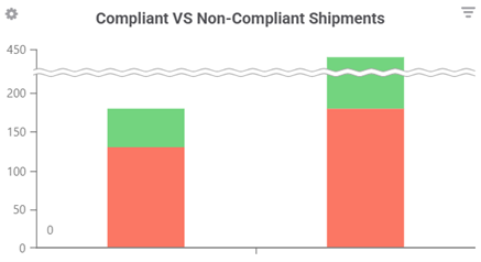
By turning complex data into simple, real-time visuals, Rebus helps teams make faster decisions that keep products moving and reduce spoilage. For example, this widget displays a few data points from multiple sites. It shows overall accuracy of shipments (how many pallets were sent correctly) as a line graph, and the red/green bar graph shows the incorrect/correct pallets shipped.
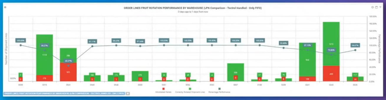
Smaller sites generally displayed fewer errors, likely due to the fact that they are easier to manage with fewer moving parts, while larger sites have more complex operations and require more resources. After seeing this data, the teams involved were able to pinpoint the problem spots and make several adjustments that reduced mistakes and made it easier to fix problems. For example, if five pallets are shipped that don’t meet a customer’s freshness requirements, the team can now quickly identify the problem and notify the customer. Using other Rebus tracking widgets on their dashboard, they can also track which pallets are affected, confirm that corrected replacements are already scheduled on an upcoming shipment, and then clearly communicate next steps to resolve the issue.
Use-Case Results#
In the previous example, after Rebus implementation company-wide, shipment accuracy increased from about 76% to 86% in just a few weeks, and with continued use and adjustments, it is now consistently staying above 95%. These numbers mean that there were fewer rejected shipments, less extra transportation and handling, and less waste. Implementation also removed most of the manual reporting work, which freed up teams to focus on more important tasks.
Aging Inventory Risk Widget#
Show how much inventory is approaching expiry or falling below the freshness window required by customers. This widget prevents waste by exposing inventory that should be shipped, reallocated, or escalated before it becomes unsellable.
Recommended Fields#
Date field (for example, report date or inventory snapshot date)
Lot or pallet identifier
Warehouse or site
Age date, receipt date, or expiry/use-by date
Customer or product freshness requirement
Steps#
Navigate to Widget Builder. Build your widget using the recommended data fields. For details on how to create widgets, refer to the Creating Widgets section of the Help Center.
At the Display Fields stage, create calculated fields such as AGE_DAYS, REMAINING_DAYS, or RISK_FLAG. Example logic: condition(lessThan(REMAINING_DAYS, REQUIRED_DAYS),1,0). This example returns if a pallet is a risk for remaining shelf life exceeding the customer requirements.
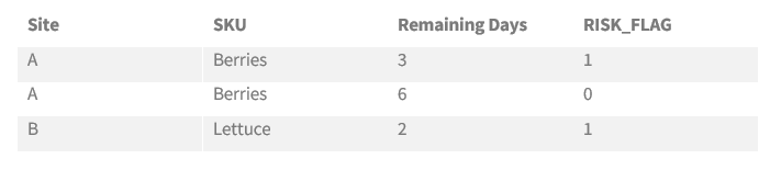
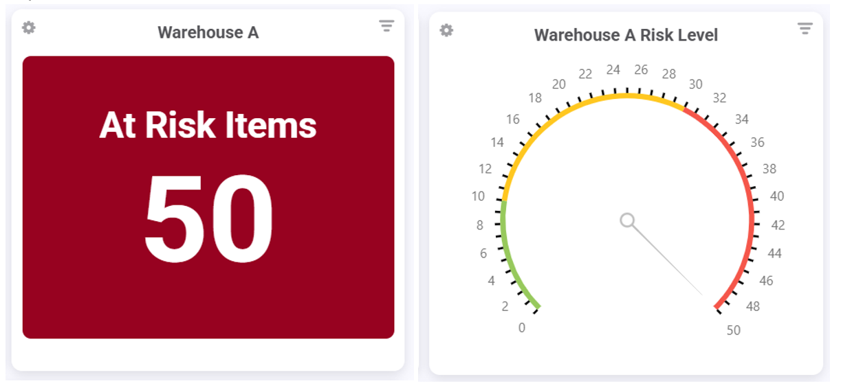
At the Grouping stage, aggregate data by site, customer, SKU, or risk if you want a summary of your data points. For example, use sum(RISK_FLAG) to summarize the total number of risky pallets per warehouse or site.

Build your widget in Chart Designer. Use a Card when leadership needs one important value, Gauge when comparing actual risk versus allowed threshold, or Grid when supervisors need the exact lots to act on.
Shipment Freshness Compliance Widget#
Track whether shipped pallets or orders met freshness requirements and which sites are driving failures. This widget helps reduce waste, rejections, and avoidable transportation costs by identifying where freshness compliance is failing so teams can take action quickly.
Recommended Fields#
Shipment date
Shipment or order identifier
Site / warehouse
Customer
Pallet or lot age at shipment
Pass/fail result or rejection reason
Correct / incorrect pallet counts
Steps#
Navigate to Widget Builder. Build your widget using the recommended data fields. For details on how to create widgets, refer to the Creating Widgets section of the Help Center.
At the Display Fields stage, create calculated fields such as PASS_FLAG and FAIL_FLAG using condition() functions. Example: condition(equals(RESULT,”PASS”),1,0). This example returns whether a shipment met freshness requirements.
At the Grouping stage, aggregate data by day, week, site, or customer depending on how you want to analyze performance.
Build your widget in Chart Designer. Use a Stacked Bar to compare compliant vs non-compliant shipments, or a Line to track compliance trends over time.
Cooling or Process Delay Widget#
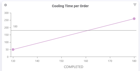
Measure the elapsed time between important events such as receipt, cooling start, cooling completion, staging, or shipment. This widget helps preserve product shelf life by identifying process bottlenecks early, allowing teams to address delays before they lead to spoilage or quality issues.
Recommended Fields#
Receipt timestamp
Cooling start/end timestamp
Site / dock / supplier / product
Elapsed time
Thresholds for time between receipt and cooling
Steps#
Navigate to Widget Builder. Build your widget using the recommended data fields. For details on how to create widgets, refer to the Creating Widgets section of the Help Center.
At the Display Fields stage, create a calculated duration field using the relevant date/time functions. Example: dateDiff(HOUR, RECEIPT_TIMESTAMP, COOLING_END_TIMESTAMP). This example calculates the total elapsed time between receipt and cooling completion.
At the Grouping stage, aggregate data by hour, day, site, or process step depending on how you want to analyze delays. For example, calculate avg(DURATION_HOURS) for average delay or count(condition(greaterThan(DURATION_HOURS, THRESHOLD),1,0)) to track records exceeding acceptable limits.
Build your widget in Chart Designer. Use a Line chart for trend monitoring over time, a Bar chart for comparing sites or process steps, or a Range chart to show minimum-to-maximum delay windows. Add a constant line to represent the maximum acceptable delay.